Callable Bond
FinPricing offers:
Four user interfaces:
- Data API.
- Excel Add-ins.
- Model Analytic API.
- GUI APP.
FinPricing provides probably the most comprehensive valuation models for financial products, including computation of:
The models calculate clean price, dirty price, accrual interest, yield to maturity, yield to call, yield to best, and yield to worst.
| 1. Callable Bond Introduction |
A callable bond is a bond in which the issuer has the right to call the bond at specified times from the investor
for a specified price.
At each callable date prior to the bond maturity, the issuer may recall the bond from its investor by returning
the investor’s money. The underlying bonds can be fixed rate bonds or
floating rate bonds. A callable bond can therefore be considered a vanilla underlying
bond with an embedded style Bermudan style option. Callable bonds protect issuers.
Therefore, a callable bond normally pays the investor a higher coupon than a non-callable bond.
Although a callable bond is a higher cost to the issuer and an uncertainty to the investor comparing to a regular
bond, it is actually quite attractive to both issuers and investors. For issuers, callable bonds
allow them to reduce interest costs at a future date should rate decrease. For investors, callable bonds allow them to
earn a higher interest rate of return until the bonds are called off. This presentation gives
an overview of callable bond and valuation model. Click the links below for details.
| 2. Callable Bond Payoffs |
Assume that the maturity of a fixed rate callable bond is T. there are n call dates denoted as .
The payoff of a callable bond at maturity is given by

The payoff of the callable bond at any call date T_i is given by

| 3. Valuation Model Selection Criteria |
Given the complexity of callable bond valuation, there is no closed form solution. Therefore, we need to select an
interest rate term structure model and a numeric solution to price Bermudan swaptions.
Popular IR term structure models in the market are Hull-White, Linear Gaussian Model (LGM), Quadratic Gaussian Model (QGM),
Heath Jarrow Morton (HJM), Libor Market Model (LMM). HJM and LMM are too complex while Hull-White is inaccurate for computing
sensitivities. Therefore, we choose either LGM or QGM.
After selecting a term structure model, we need to choose a numeric approach to approximate the underlying stochastic
process of the model.Commonly used numeric approaches are tree, partial differential equation (PDE), lattice, and Monte Carlo
simulation. Tree and Monte Carlo are notorious for inaccuracy in sensitivity calculation. Therefore, we choose either PDE
or lattice. Our final decision is to use LGM plus lattice.
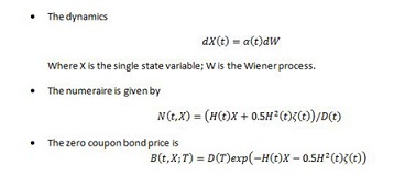
| 4. LGM Model |

| 5. LGM Assumptions and Calibration |
The LGM model is mathematically equivalent to the Hull-White model but offers significant improvements in calibration
stability and accuracy. It is also more accurate and stable in sensitivity calculation. The state variable is normally
distributed under the appropriate measure. The LGM model has only one stochastic driver (one-factor), thus changes in rates
are perfected correlated.
At time t, X(0)=0 and H(0)=0. Thus Z(0,0;T)=D(T). In other words, the LGM automatically fits today’s
discount curve or yield curve. To calibrate
swaption implied volatilities, first select a group of market
swaptions and then solve parameters by minimizing the relative error between the market
swaption prices and the LGM model swaption prices.
| 5. Valuation Practical Guide |
| References |